Pollen Classification
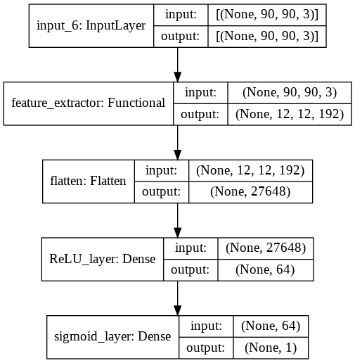
This post shows how to train a convolutional network for pollen classification. We used part of the MobileNetV2 network for feature extraction and one ReLU layer with one sigmoid layer for classification.
Dependecies
import numpy as np
import pandas as pd
import matplotlib.pyplot as plt
import tensorflow as tf

from tensorflow.keras.models import Model
from tensorflow.keras.layers import Flatten, Dense, Input
from tensorflow.keras.applications import MobileNetV2
from tensorflow_addons.metrics import F1Score
from sklearn.metrics import classification_report, confusion_matrix, ConfusionMatrixDisplay
Dataset Functions
Here we are using the tf.keras.preprocessing.image_dataset_from_directory function to load the dataset from the images/ directory. The labels of the images are inferred by the name of the folder that contains them.
images/
...NP/
......a_image_1.jpg
......a_image_2.jpg
...P/
......b_image_1.jpg
......b_image_2.jpg
def normalize_image(image,label):
    image = tf.cast(image/255. ,tf.float32)
    return image,label

train_dataset = tf.keras.preprocessing.image_dataset_from_directory(
    "images/",
    labels="inferred",
    label_mode="binary",
    color_mode="rgb",
    batch_size=32,
    image_size=(90, 90),
    shuffle=True,
    seed=42,
    validation_split=0.2,
    subset="training"
).map(normalize_image)

valid_dataset = tf.keras.preprocessing.image_dataset_from_directory(
    "images/",
    labels="inferred",
    label_mode="binary",
    color_mode="rgb",
    batch_size=32,
    image_size=(90, 90),
    shuffle=True,
    seed=42,
    validation_split=0.2,
    subset="validation",
).map(normalize_image)
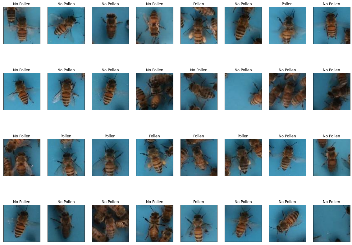
Here we plot some examples to see how are the images in this dataset. We can identify variations on bee pose and size, illumination, rotation and etc.
fig, ax = plt.subplots(4, 8, figsize=(20, 15))
axes = ax.ravel()

gen = iter(train_dataset)
sample_batch = next(gen)

for i, (image, label) in enumerate(zip(sample_batch[0], sample_batch[1])):
    axes[i].imshow(image)
    label_str = "Pollen" if label[0] else "No Pollen"
    axes[i].set_title("{}".format(label_str))
    axes[i].set_xticks([])
    axes[i].set_yticks([])
MobileNetV2 as Feature extractor
In this notebook we are using a MobileNetV2 which comes with keras. You can find other pre-made models on tf.keras.applications. More details about the models here. We cut the network at the layer block_6 to have a resolution of 12x12 for the features.
backbone = MobileNetV2(include_top=False, input_shape=(90, 90, 3))
model_input = backbone.input
model_out = backbone.get_layer("block_6_expand_relu").output
feature_extractor = Model(model_input, model_out)
Classification Layer
class Classifier(tf.keras.Model):
    def __init__(self, base_model, filters=64, classes=2):
        super(Classifier, self).__init__()
        self.backbone = base_model
        self.flatten = Flatten(name='flatten')
        self.dense = Dense(filters,activation='relu', name="ReLU_layer")
        if classes == 1:
            self.classifier = Dense(classes, activation="sigmoid", name="sigmoid_layer")
        else:
            self.classifier = Dense(classes, activation="softmax")
        self.model_name = "Classifier"

    def call(self, data):
        x = data
        x = self.backbone(x)
        x = self.flatten(x)
        x = self.dense(x)
        id_class = self.classifier(x)
        return id_class


model = Classifier(feature_extractor, classes=1)
Model Training
The optimization loss of this model is the binary cross-entropy.
\[loss = - \frac{1}{N} \sum_i^N y_i \log{\hat{y}_i} + (1 - y_i) \log (1 - \hat{y}_i)\]model.compile(loss='binary_crossentropy', optimizer="adam",metrics=['accuracy', F1Score(num_classes=1, threshold=0.5)])
We used F1Score metric to have a good idea of the performance of the model because our pollen dataset is unbalanced (we have a lot more images labeled as No pollen than Pollen.)
history = model.fit(train_dataset, epochs=20, validation_data=valid_dataset)
history_df = pd.DataFrame(history.history, index=history.epoch)
Epoch 1/20
140/140 [==============================] - 12s 67ms/step - loss: 0.5654 - accuracy: 0.9096 - f1_score: 0.8008 - val_loss: 0.6154 - val_accuracy: 0.8317 - val_f1_score: 0.4689
Epoch 2/20
140/140 [==============================] - 9s 63ms/step - loss: 0.0517 - accuracy: 0.9839 - f1_score: 0.9656 - val_loss: 0.5985 - val_accuracy: 0.8335 - val_f1_score: 0.4775
Epoch 3/20
140/140 [==============================] - 9s 62ms/step - loss: 0.0241 - accuracy: 0.9915 - f1_score: 0.9819 - val_loss: 0.3709 - val_accuracy: 0.9042 - val_f1_score: 0.7540
Epoch 4/20
140/140 [==============================] - 9s 63ms/step - loss: 0.0071 - accuracy: 0.9987 - f1_score: 0.9972 - val_loss: 0.3563 - val_accuracy: 0.9141 - val_f1_score: 0.7848
Epoch 5/20
140/140 [==============================] - 9s 63ms/step - loss: 0.0074 - accuracy: 0.9975 - f1_score: 0.9948 - val_loss: 0.3406 - val_accuracy: 0.9096 - val_f1_score: 0.7710
Epoch 6/20
140/140 [==============================] - 9s 61ms/step - loss: 0.0034 - accuracy: 0.9996 - f1_score: 0.9991 - val_loss: 0.4709 - val_accuracy: 0.8962 - val_f1_score: 0.7277
Epoch 7/20
140/140 [==============================] - 9s 62ms/step - loss: 8.3022e-04 - accuracy: 1.0000 - f1_score: 1.0000 - val_loss: 0.3459 - val_accuracy: 0.9194 - val_f1_score: 0.8009
Epoch 8/20
140/140 [==============================] - 9s 64ms/step - loss: 2.3191e-04 - accuracy: 1.0000 - f1_score: 1.0000 - val_loss: 0.2589 - val_accuracy: 0.9364 - val_f1_score: 0.8493
Epoch 9/20
140/140 [==============================] - 9s 62ms/step - loss: 1.4356e-04 - accuracy: 1.0000 - f1_score: 1.0000 - val_loss: 0.2349 - val_accuracy: 0.9409 - val_f1_score: 0.8613
Epoch 10/20
140/140 [==============================] - 9s 63ms/step - loss: 9.4333e-05 - accuracy: 1.0000 - f1_score: 1.0000 - val_loss: 0.1998 - val_accuracy: 0.9508 - val_f1_score: 0.8871
Epoch 11/20
140/140 [==============================] - 9s 62ms/step - loss: 8.5224e-05 - accuracy: 1.0000 - f1_score: 1.0000 - val_loss: 0.1852 - val_accuracy: 0.9552 - val_f1_score: 0.8984
Epoch 12/20
140/140 [==============================] - 9s 62ms/step - loss: 6.3893e-05 - accuracy: 1.0000 - f1_score: 1.0000 - val_loss: 0.1726 - val_accuracy: 0.9597 - val_f1_score: 0.9095
Epoch 13/20
140/140 [==============================] - 9s 62ms/step - loss: 5.8994e-05 - accuracy: 1.0000 - f1_score: 1.0000 - val_loss: 0.1611 - val_accuracy: 0.9624 - val_f1_score: 0.9160
Epoch 14/20
140/140 [==============================] - 9s 63ms/step - loss: 4.3215e-05 - accuracy: 1.0000 - f1_score: 1.0000 - val_loss: 0.1542 - val_accuracy: 0.9642 - val_f1_score: 0.9203
Epoch 15/20
140/140 [==============================] - 9s 63ms/step - loss: 5.1431e-05 - accuracy: 1.0000 - f1_score: 1.0000 - val_loss: 0.1408 - val_accuracy: 0.9678 - val_f1_score: 0.9289
Epoch 16/20
140/140 [==============================] - 9s 62ms/step - loss: 3.9965e-05 - accuracy: 1.0000 - f1_score: 1.0000 - val_loss: 0.1428 - val_accuracy: 0.9678 - val_f1_score: 0.9289
Epoch 17/20
140/140 [==============================] - 9s 63ms/step - loss: 3.5314e-05 - accuracy: 1.0000 - f1_score: 1.0000 - val_loss: 0.1373 - val_accuracy: 0.9687 - val_f1_score: 0.9310
Epoch 18/20
140/140 [==============================] - 9s 62ms/step - loss: 2.9370e-05 - accuracy: 1.0000 - f1_score: 1.0000 - val_loss: 0.1386 - val_accuracy: 0.9696 - val_f1_score: 0.9331
Epoch 19/20
140/140 [==============================] - 9s 63ms/step - loss: 2.4445e-05 - accuracy: 1.0000 - f1_score: 1.0000 - val_loss: 0.1319 - val_accuracy: 0.9696 - val_f1_score: 0.9331
Epoch 20/20
140/140 [==============================] - 9s 63ms/step - loss: 2.5461e-05 - accuracy: 1.0000 - f1_score: 1.0000 - val_loss: 0.1306 - val_accuracy: 0.9722 - val_f1_score: 0.9393
Check Training
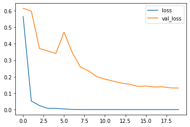
Seems that our model is not overfitting both training and validation curves decrease over time.
plt.plot(history_df["loss"], label="loss");
plt.plot(history_df["val_loss"], label="val_loss");
plt.legend();
y_pred = []  # store predicted labels
y_true = []  # store true labels
X_valid = [] # store the image

for image_batch, label_batch in valid_dataset:
    X_valid.append(image_batch)

    y_true.append(label_batch)
    # compute predictions
    preds = model.predict(image_batch)
    # append predicted labels
    y_pred.append(preds)

# convert the true and predicted labels into tensors
correct_labels = tf.concat([item for item in y_true], axis = 0)
predicted_labels = tf.concat([item for item in y_pred], axis = 0)
images = tf.concat([item for item in X_valid], axis = 0)
cm = confusion_matrix(correct_labels, predicted_labels > 0.5, normalize='all')
ConfusionMatrixDisplay(cm, display_labels=["No Pollen", "Pollen"]).plot()
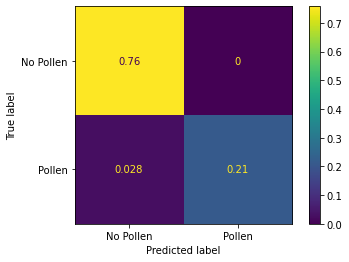
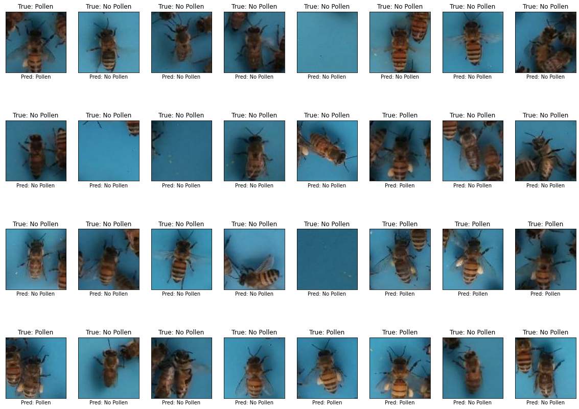
From the confussion matrix we can see that our model do not have false positives. There some false negatives but in general our pollen model is very accurate. Also, we can see that our validation dataset is unbalanced where 76% of the data belongs to No pollen class.
print(classification_report(correct_labels, predicted_labels > 0.5 ))
              precision    recall  f1-score   support

         0.0       0.96      1.00      0.98       846
         1.0       1.00      0.89      0.94       271

    accuracy                           0.97      1117
   macro avg       0.98      0.94      0.96      1117
weighted avg       0.97      0.97      0.97      1117
Check Predictions
random_idx = np.random.permutation(len(images))
random_idx = random_idx[:32]
fig, ax = plt.subplots(4, 8, figsize=(20, 15))
axes = ax.ravel()

for i, idx in enumerate(random_idx):
    axes[i].imshow(images[idx])
    true_label = "Pollen" if correct_labels[idx] > 0.5 else "No Pollen"
    pred_label = "Pollen" if predicted_labels[idx] > 0.5 else "No Pollen"

    title = true_label + pred_label
    axes[i].set_title("True: {}".format(true_label))
    axes[i].set_xlabel("Pred: {}".format(pred_label))
    axes[i].set_xticks([])
    axes[i].set_yticks([])
Check Hard Cases
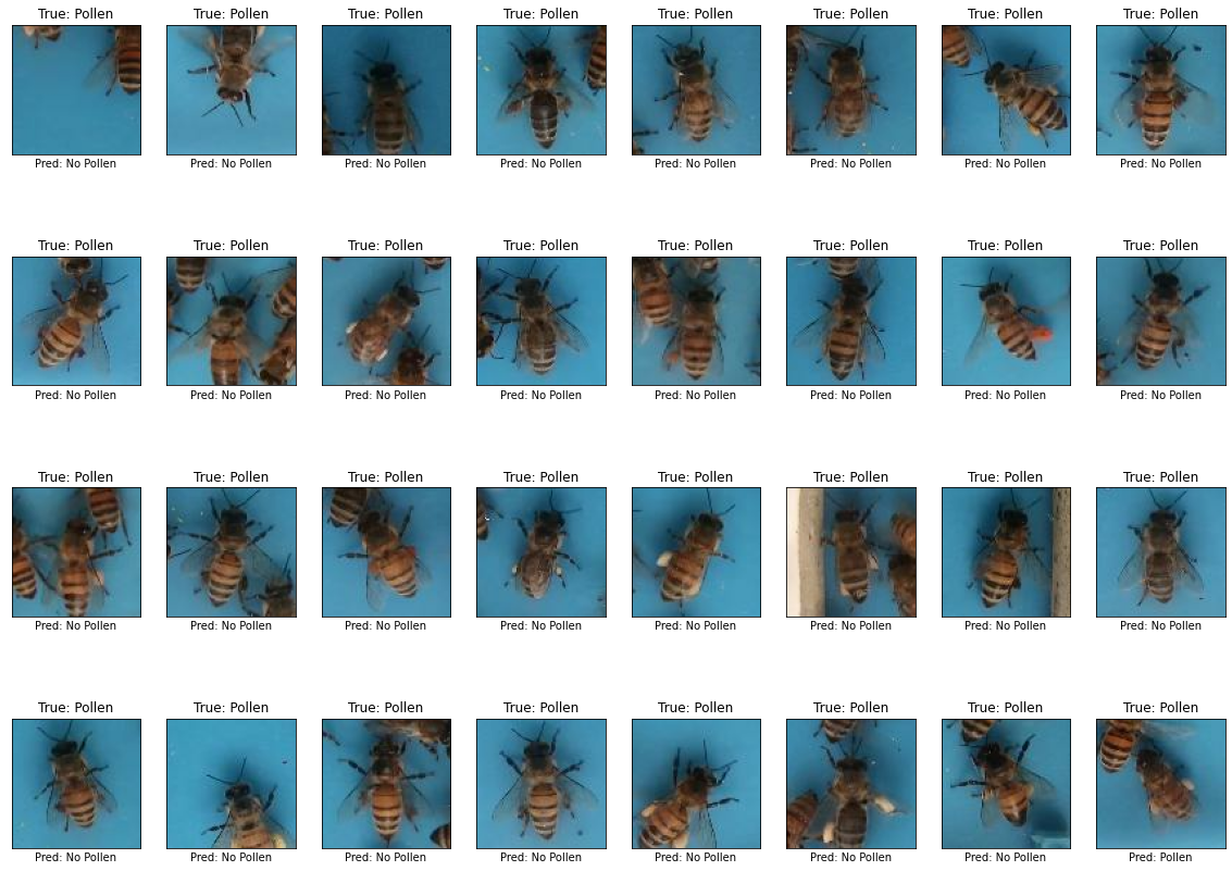
To plot the hard cases we sorted the errors in descending order and plot the top 32 images with greater error. Plotting the hard cases we can see our model false negatives. Some of the examples seems hard even for humans.
errors = (correct_labels - predicted_labels)**2
hard_cases_indxes = tf.argsort(errors, direction="DESCENDING", axis=0)
hard_cases_indxes = tf.reshape(hard_cases_indxes, -1)

fig, ax = plt.subplots(4, 8, figsize=(20, 15))
axes = ax.ravel()

for i, idx in enumerate(hard_cases_indxes[:32]):
    axes[i].imshow(images[idx])
    true_label = "Pollen" if correct_labels[idx] > 0.5 else "No Pollen"
    pred_label = "Pollen" if predicted_labels[idx] > 0.5 else "No Pollen"

    title = true_label + pred_label
    axes[i].set_title("True: {}".format(true_label))
    axes[i].set_xlabel("Pred: {}".format(pred_label))
    axes[i].set_xticks([])
    axes[i].set_yticks([])
Conclusion
We trained our pollen model using the Tensorflow/Keras framework. We obtained a very accurate model without any false positive case on the validation dataset, but with few false negatives examples. Some of these false negatives examples are hard even for humans.